Exploring

An exoplanet Population is designed to be a (hopefully!) relatively easy way to interact with data for a group of exoplanet systems. Here we step through the basics of how we can explore a population of planets, access standardized planet properties, and filter subsets of planet populations.

Getting started

The exoatlas package contains the tools we will use. All planet properties inside a population have astropy units associated with them, so we make also want to have access to those units for our calculations.

import exoatlas as ea
import astropy.units as u

We can always check what version of exoatlas we’re using with its hidden .__version__.

ea.__version__

'0.2.4'

Create a Population

Now, to get started, we’ll make a population that contains all confirmed transiting exoplanets. We can read more about the different populations we can create over one the Creating page. When we create this population, the code will download a table of the latest data from the NASA Exoplanet Archive.

pop = ea.TransitingExoplanets()

/Users/zkbt/.exoatlas/data/standardized-TransitingExoplanets.txt is 0.009 days old.
Should it be updated? [y/N]
[transitingexoplanets] Loaded standardized table from /Users/zkbt/.exoatlas/data/standardized-TransitingExoplanets.txt

(The code will let you know how long ago your local dataset was updated, and ask if you’d like to update it now.)

What’s inside a Population?

The core ingredient to an exoplanet Population is a table of planet properties that have been standardized and populated with astropy units. This pop.standard table is an astropy Table, so its contents can be accessed or modified as any other astropy Table.

pop.standard

Table length=3135

name	ra	dec	period	semimajoraxis	e	omega	inclination	transit_epoch	transit_duration	transit_depth	stellar_teff	stellar_radius	stellar_mass	UJmag	VJmag	BJmag	RCmag	ICmag	Jmag	Hmag	Kmag	WISE1mag	WISE2mag	WISE3mag	WISE4mag	radius	radius_uncertainty_upper	radius_uncertainty_lower	transit_ar	transit_b	rv_semiamplitude	mass	mass_uncertainty_upper	mass_uncertainty_lower	distance	distance_uncertainty_upper	distance_uncertainty_lower	discoverer
	deg	deg	d	AU		deg	deg	d	d		K	solRad	solMass													earthRad	earthRad	earthRad				earthMass	earthMass	earthMass	pc	pc	pc
str17	float64	float64	float64	float64	float64	float64	float64	float64	float64	float64	float64	float64	float64	float64	float64	float64	float64	float64	float64	float64	float64	float64	float64	float64	float64	float64	float64	float64	float64	float64	float64	float64	float64	float64	float64	float64	float64	str44
55Cnce	133.149216	28.330818	0.736539	0.01544	nan	nan	83.3	2455733.013	nan	nan	5196.0	0.94	0.91	nan	5.96	6.83	nan	nan	4.768	4.265	4.015	4.001	3.296	4.051	4.014	1.91	0.08	-0.08	nan	0.41	nan	8.08	0.31	-0.31	12.59	0.01	-0.01	McDonald Observatory
BD+20594b	53.650967	20.599232	41.6855	nan	0.0	nan	89.55	nan	nan	0.00049	5766.0	1.08	1.67	nan	11.038	11.728	nan	nan	9.77	9.432	9.368	9.31	9.344	9.332	8.976	2.578	0.112	-0.112	55.8	nan	3.1	22.2481	9.5349	-9.5349	180.39	1.25	-1.25	K2
CoRoT-10b	291.063708	0.746143	13.2406	0.1055	0.53	218.9	88.55	2454273.3436	0.1242	0.0161036	5075.0	0.79	0.89	nan	15.22	16.68	nan	nan	12.527	11.929	11.782	11.64	11.752	11.396	8.923	10.87	0.78	-0.78	31.33	0.85	301.0	874.0	50.85	-50.85	345.0	70.0	-70.0	CoRoT
CoRoT-11b	280.687263	5.937688	2.99433	0.0436	0.0	nan	83.17	2454597.679	0.1042	0.011449	6440.0	1.37	1.27	nan	12.939	13.596	nan	nan	11.589	11.416	11.248	11.173	11.265	11.47	9.198	16.03	0.34	-0.34	6.89	0.818	280.0	740.51	108.06	-108.06	560.0	30.0	-30.0	CoRoT
CoRoT-12b	100.765677	-1.296439	2.828042	0.04016	0.07	105.0	85.48	2454398.62707	0.10726	0.01744	5675.0	1.12	1.08	nan	15.515	16.343	nan	nan	14.024	13.63	13.557	13.47	13.47	12.53	8.61	16.14	1.46	-1.46	nan	0.573	125.5	291.438	22.247	-20.658	1150.0	85.0	-85.0	CoRoT
CoRoT-13b	102.721137	-5.086445	4.03519	0.051	0.0	nan	88.02	2454790.8091	0.1308	nan	5945.0	1.01	1.09	nan	15.039	15.777	nan	nan	13.71	13.406	13.376	13.17	13.217	12.615	8.946	9.92	0.157	-0.157	10.81	0.374	157.8	415.704	20.976	-20.976	1060.0	100.0	-100.0	CoRoT
CoRoT-14b	103.424211	-5.536037	1.51214	0.027	0.0	nan	79.6	2454787.6694	0.0693	nan	6035.0	1.21	1.13	nan	16.033	16.891	nan	nan	14.321	14.007	13.806	13.679	13.729	12.03	9.14	12.22	0.78	-0.78	4.78	0.86	1230.0	2415.4	190.7	-190.7	1340.0	110.0	-110.0	CoRoT
CoRoT-16b	278.524691	-6.002595	5.35227	0.0618	0.33	168.41	85.01	2454923.9138	0.0996	0.0102	5650.0	1.19	1.1	nan	15.63	16.68	nan	nan	13.496	12.98	12.847	nan	nan	nan	nan	13.11	1.79	-1.57	11.2	0.825	61.96	170.032	27.014	-26.379	840.0	90.0	-90.0	CoRoT
CoRoT-17b	278.699254	-6.612234	3.7681	0.0461	0.0	0.0	88.34	2454923.3093	0.196667	0.0044	5740.0	1.59	1.04	nan	15.46	nan	nan	nan	13.174	12.615	12.472	nan	nan	nan	nan	11.43	0.78	-0.78	6.23	0.18	312.4	772.29	95.34	-95.34	920.0	50.0	-50.0	CoRoT
...	...	...	...	...	...	...	...	...	...	...	...	...	...	...	...	...	...	...	...	...	...	...	...	...	...	...	...	...	...	...	...	...	...	...	...	...	...	...
WTS-1b	293.9932	36.290325	3.352057	0.047	0.1	nan	85.5	2454318.7472	nan	0.017636	6250.0	1.15	1.2	nan	16.13	nan	nan	nan	15.375	15.187	15.271	nan	nan	nan	nan	16.7	1.79	-2.02	nan	0.69	nan	1274.44	111.24	-111.24	3200.0	900.0	-400.0	United Kingdom Infrared Telescope
WTS-2b	293.732796	36.815491	1.0187068	0.01855	0.0	nan	83.55	2454317.81333	nan	nan	5000.0	0.75	0.82	nan	15.9	16.8	nan	nan	13.928	13.464	13.414	13.299	13.367	12.107	9.176	15.278	0.684	-0.684	nan	0.584	256.0	355.9696	50.8528	-50.8528	1000.0	nan	nan	United Kingdom Infrared Telescope
Wolf503b	206.847687	-6.136875	6.00118	0.0571	nan	nan	nan	2458185.36087	0.0550417	nan	4716.0	0.69	0.69	nan	10.26	11.27	nan	9.09	8.324	7.774	7.617	nan	nan	nan	nan	2.03	0.076	-0.073	nan	0.387	nan	nan	inf	inf	44.58	0.1	-0.1	K2
XO-1b	240.54935	28.169586	3.94153	nan	0.0	nan	88.81	nan	nan	0.018000000000000002	5750.0	0.88	0.88	nan	11.19	11.85	10.81	10.43	9.939	9.601	9.527	9.495	9.518	9.507	9.248	12.778	0.785	-0.785	11.37	nan	116.0	263.7989	41.3179	-41.3179	164.33	0.62	-0.62	XO
XO-2Nb	117.026968	50.2258	2.61586178	0.0368	nan	nan	88.01	2454508.73829	0.1118292	nan	5307.0	0.99	0.97	nan	11.138	12.002	10.669	10.243	9.744	9.34	9.308	9.24	9.31	9.236	8.833	11.131	0.135	-0.135	7.986	0.28	nan	179.89178	7.94575	-7.94575	154.94	1.45	-1.45	XO
XO-3b	65.469581	57.817181	3.19154	nan	0.29	nan	79.32	nan	nan	0.0089	6429.0	1.54	0.58	nan	9.8	10.25	nan	nan	9.013	8.845	8.791	8.754	8.765	8.736	8.372	15.805	1.345	-1.345	4.95	nan	1488.0	2316.9807	378.2177	-378.2177	214.31	2.7	-2.7	XO
XO-4b	110.388223	58.268108	4.12508	nan	0.0	nan	88.8	nan	nan	0.0078000000000000005	6397.0	1.45	1.1	nan	10.674	11.24	nan	nan	9.667	9.476	9.406	9.373	9.398	9.378	8.716	14.011	0.897	-0.897	7.68	nan	168.6	451.3186	60.3877	-60.3877	274.79	2.91	-2.91	XO
XO-5b	116.716527	39.094578	4.1877558	0.0515	0.0	nan	86.8	2456864.3129	0.1299	0.0108	5430.0	1.13	1.04	nan	12.13	nan	nan	nan	10.774	10.443	10.345	10.333	10.381	10.292	8.354	12.78	0.34	-0.34	nan	0.55	146.0	378.2	9.53	-9.53	278.37	3.9	-3.9	XO
XO-6b	94.793282	73.827682	3.7650007	0.0815	0.0	nan	86.0	2456652.71245	0.1208333	nan	6720.0	1.93	1.47	nan	10.25	nan	nan	nan	9.471	9.266	9.246	9.213	9.232	9.34	8.709	23.203	2.466	-2.466	9.08	0.633	450.0	1398.452	inf	inf	237.06	2.43	-2.43	XO
piMenc	84.291214	-80.469124	6.2679	0.06839	0.0	nan	87.456	2458325.504	0.1230417	0.0003	6037.0	1.1	1.09	6.36	5.67	6.25	nan	nan	4.869	4.424	4.241	4.269	3.972	4.199	4.219	2.042	0.05	-0.05	13.38	0.59	1.58	4.82	0.84	-0.86	18.28	0.02	-0.02	Transiting Exoplanet Survey Satellite (TESS)

If desired, columns could be added to this standardized table:

import numpy as np
N = len(pop)
pop.standard['something'] = np.arange(N) + 5

How do we access planet properties?

The main way to access planet properties within a Populatoin is with its attributes. That is, we can access an array of the values for some property x by calling pop.x. Behind the scenes, the population will look to see if there is a column called "x" in the standardized table and return that column. For example, we can get an array of planet names with:

pop.name

array(['55Cnce', 'BD+20594b', 'CoRoT-10b', ..., 'XO-5b', 'XO-6b',
       'piMenc'], dtype='<U17')

Even columns that we separately added to the standardized table can be accessed as attributes:

pop.something

$[ 5,~ 6,~ 7,~\dots,~3137,~3138,~3139] \; \mathrm{}$

We also have access to quantities that are not directly included in the table itself but can be calculated from them. For example, we can get an array of the amount of insolation that the planets receive from their stars as:

pop.insolation

[transitingexoplanets] 1626/3135 semimajoraxes are missing
[transitingexoplanets] 0/3135 are still missing after NVK3L

$[3313157.1,~20290.402,~45613.962,~\dots,~513270.26,~1402428.9,~421394.84] \; \mathrm{\frac{W}{m^{2}}}$

In this case, the insolation is calculated from the planet’s orbital separation and the luminosity of the star (which is itself calculated from the stellar effective temperature and radius).

If information needed to do a calculation is missing, exoatlas will try to estimate them from other available information. In the .insolation case, some planets had no semimajor axes defined in the .standard table, but we were able to calculate this quantity from the orbital period, the stellar mass, and Newton’s Version of Kepler’s 3rd Law.

Short descriptions of some common attributes can printed with the describe_columns() function.

ea.describe_columns()

               name = name of the planet
                 ra = Right Ascension of the system
                dec = Declination of the system
           distance = distance to the system
   distance_modulus = apparent magnitude - absolute magnitude
         discoverer = telescope/project that found this planet
       stellar_teff = stellar effective temperature
       stellar_mass = stellar mass
     stellar_radius = stellar radius
 stellar_luminosity = luminosity of the star
 stellar_brightness = photon flux from the star at Earth (a function of wavelength)
             period = orbital period of the planet
      semimajoraxis = the semimajor axis of the planet's orbit
          a_over_rs = scaled orbital distance a/R*
                  b = impact parameter b
                  e = eccentricity
              omega = argument of periastron
             radius = planet radius
               mass = planet mass
            density = density of the planet
         insolation = bolometric energy flux the planet receives from its star
relative_insolation = insolation relative to Earth
                teq = equilibrium temperature of the planet (assuming 0 albedo)
    surface_gravity = surface gravity of the planet
       scale_height = scale height of an H2-rich atmosphere
    escape_velocity = escape velocity of the planet
   escape_parameter = ratio of gravitational potential to thermal energy for an H atom
      transit_epoch = a transit midpoint
   transit_duration = duration of the transit
      transit_depth = fraction of starlight the planet blocks
         transit_ar = (transit-derived) scaled orbital distance a/R*
          transit_b = (transit-derived) impact parameter b
transmission_signal = transit depth of one scale height of atmosphere
    emission_signal = thermal-emission eclipse depth (a function of wavelength)
  reflection_signal = reflected-light eclipse depth (for an albedo of 1)

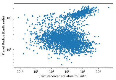
With this toolkit, you can now access the data you need to make some pretty fundamental plots in exoplanetary science. For example:

import matplotlib.pyplot as plt
plt.loglog(pop.relative_insolation, pop.radius, '.')
plt.xlabel('Flux Received (relative to Earth)')
plt.ylabel('Planet Radius (Earth radii)');

[transitingexoplanets] 1626/3135 semimajoraxes are missing
[transitingexoplanets] 0/3135 are still missing after NVK3L

How do we access some sub-population of planets?

Often we’ll want to pull out some subset of a population. We might want a smaller sample of planets, or all the planets that meet some particular criterion, or maybe the properties of one individual planet. In our experience with numpy arrays or astropy tables, we’ve often done this by indexing (x[0] or x[[0, 1, 5]]), slicing (x[3:30]), or masking (x[some_array > some_other_array]).

We can apply the same methods to a Population, creating smaller populations by indexing, slicing, or masking. Anything we can do with a Population we can do with one of these sub-Populations that we create.

pop

<Transiting Exoplanets | population of 3135 planets>

one_planet = pop[0]
one_planet

<ExoplanetSubsets of Transiting Exoplanets | population of 1 planets>

one_planet.name, one_planet.radius, one_planet.insolation

   [population] 0/1 semimajoraxes are missing
   [population] 0/1 are still missing after NVK3L

(array(['55Cnce'], dtype='<U17'),
 <Quantity [1.91] earthRad>,
 <Quantity [3313157.14969688] W / m2>)

prime_planets = pop[[2, 3, 5, 7, 11, 13, 17, 19, 23]]
prime_planets

<ExoplanetSubsets of Transiting Exoplanets | population of 9 planets>

first_ten = pop[:10]
first_ten

<ExoplanetSubsets of Transiting Exoplanets | population of 10 planets>

every_other_exoplanet = pop[::2]
every_other_exoplanet

<ExoplanetSubsets of Transiting Exoplanets | population of 1568 planets>

small = pop[pop.radius < 4*u.Rearth]
small

<ExoplanetSubsets of Transiting Exoplanets | population of 2433 planets>

Additionally, we can extract an individual planet or a list of planets by indexing the population with planet name(s). This is using astropy tables’ .loc functionality, with "name" being used as an index.

cute_planet = pop['GJ 1214b']
cute_planet

<ExoplanetSubsets of Transiting Exoplanets | population of 1 planets>

cute_planets = pop[['LHS 1140b', 'GJ 1214b', 'GJ 436b']]
cute_planets

<ExoplanetSubsets of Transiting Exoplanets | population of 3 planets>

Explore!

That’s about it. For more information about different pre-defined populations see Creating, and for more about pre-packaged visualizations see Visualizing.