Let’s start from all the transiting exoplanets in the NASA Exoplanet Archive, and then filter down into a Population of planets we might want to consider observing.
import exoatlas as ea
import exoatlas.visualizations as vi

ea.version()'1.0.0'Download Exoplanet Data
Let’s download a recent list of transiting exoplanets from the NASA Exoplanet Archive. We should, as always, be careful not to completely trust every detail of this database. For any particular planet, there’s a possibility that details might be wrong or missing so for anything super crucial, it would be very wise to double check.
e = ea.TransitingExoplanets()
s = ea.SolarSystem()
Throughout, let’s use PlanetGallery to visualize how the various filtering cuts remove planets from our observing sample.
vi.PlanetGallery().build(e);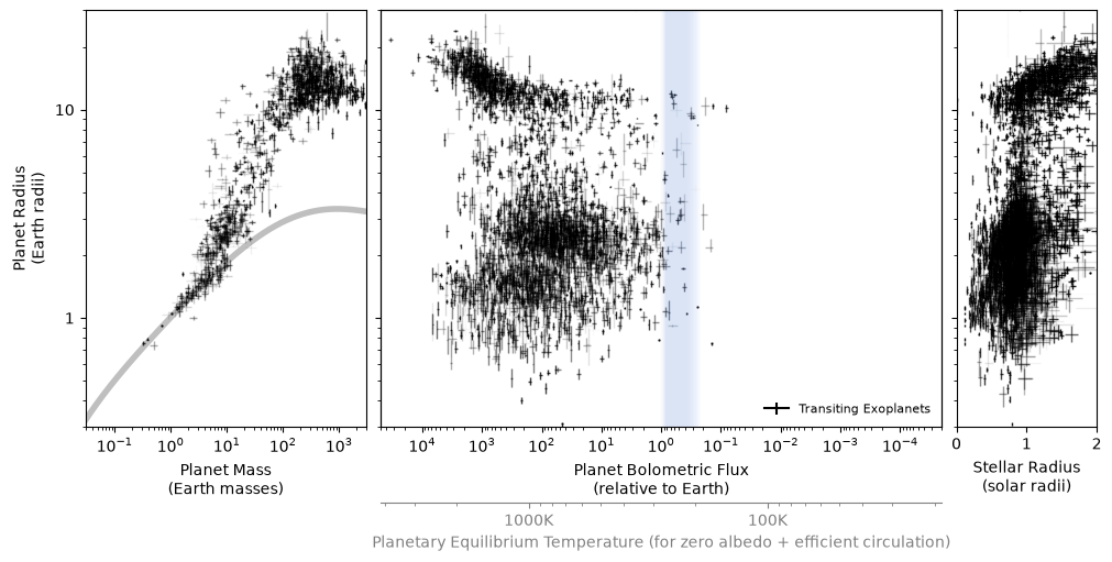
Define Filtering Criteria
Let’s make some cuts to this sample in order to select systems that might be worth trying to observe at the telescope. We’ll start by defining an unfiltered population, for comparison.
unfiltered = e[:]
unfiltered.color = "orchid"
unfiltered.label = "Unfiltered"
Is it big enough?
To ensure that a planet has a hydrogen-dominated atmosphere (which makes interpreting a transmission spectrum a lot easier), we could place a cut on the planet’s radius. “Most 1.6 Earth-radius planets are not rocky”, so let’s try cutting there.
import astropy.units as u

is_big = e.radius() > 1.6 * u.Rearth
filtered = e[is_big]
filtered.label = "Big"
filtered
✨ Big | 3342 elements ✨vi.PlanetGallery().build([unfiltered, filtered]);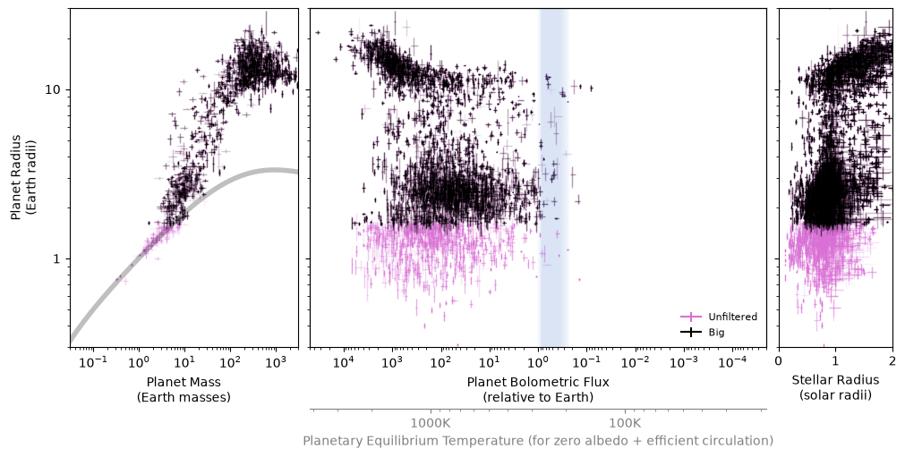
Is the duration short enough?
An ideal transit observation would include at least some baseline before the start and after the end of the transit itself. When observing from a ground-based telescope, practically that means it’s really hard to observe (complete) transits with durations longer than about a few hours.
is_short = e.transit_duration() < 3 * u.hour
filtered = e[is_short]
filtered.label = "Short"
filtered
✨ Short | 2185 elements ✨vi.PlanetGallery().build([unfiltered, filtered]);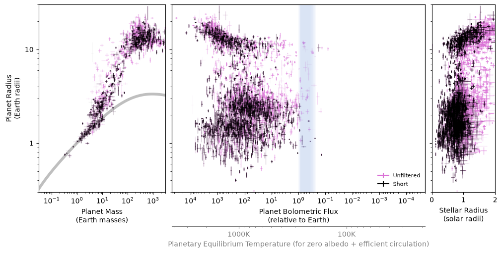
Is transmission spectroscopy possible?
The best precision we could possibly achieve on measuring a transit depth is set by the number of photons that we can gather with our telescope. If the signal we’re hoping to detect for transmission spectroscopy (see Observing) is smaller than that expected precision, it’s basically hopeless that we’ll see anything. So, let’s at least limit our sample to targets with a reasonably high predicted signal-to-noise ratio.
import matplotlib.pyplot as plt
import numpy as np

signal = e.transmission_signal()
wavelength = 0.7 * u.micron
dt = 1 * u.hour
R = 10
noise = e.depth_uncertainty(telescope="APO", wavelength=wavelength, dt=dt, R=R)
snr = signal / noise

plt.figure(figsize=(8, 5))
plt.scatter(noise, signal, c=snr, vmin=1, vmax=10)
plt.xscale("log")
plt.yscale("log")
plt.axis("scaled")
plt.xlabel("")
plt.ylim(1e-6, 1e-2)
plt.xlim(1e-6, 1e-2)
plt.plot(
    [1e-6, 1e-2], [1e-6, 1e-2], color="black", linewidth=3, linestyle="--", alpha=0.3
)
plt.colorbar(label="S/N")
plt.xlabel(rf"Predicted Photon Noise\n($\lambda=${wavelength}, dt={dt}, R={R})")
plt.ylabel(r"Possible Transmission\nSignal Size ($2HR_p/R_{\star}^2$)");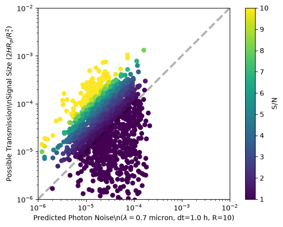
is_snr = snr > 5
filtered = e[is_snr]
filtered.label = "High S/N"
filtered
✨ High S/N | 289 elements ✨vi.PlanetGallery().build([unfiltered, filtered]);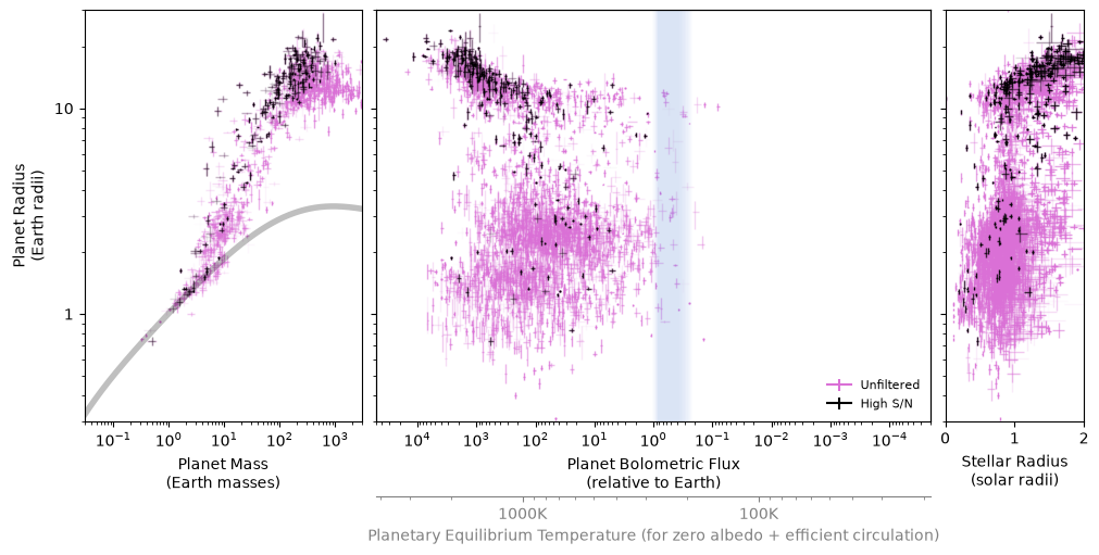
Is it above the horizon at night?
If we’re observing at a particular time of year from a particular observatory, only some targets will be high enough in the sky to be observable at night. Let’s place a cut on the airmass at midnight on some particular night, so we don’t waste time considering planets that are beneath the Earth when we might be trying to observe.
from astroplan import Observer
from astropy.time import Time

date = Time.now()
observatory = Observer.at_site("APO", timezone="US/Mountain")
local_midnight = observatory.midnight(date)
sidereal_time_at_midnight = observatory.local_sidereal_time(local_midnight)
ra_at_midnight = sidereal_time_at_midnight
ra_at_midnightdeclination_at_zenith = observatory.latitude
declination_at_zenithairmass = e.airmass(where=observatory, when=local_midnight)
is_up = airmass < 2
filtered = e[is_up]
filtered.name = "Up at Midnight"
plt.figure()
plt.scatter(e.ra(), e.dec(), color="black", marker=".", s=2, alpha=0.2)
plt.scatter(filtered.ra(), filtered.dec(), color="black", marker="o", facecolor="none")
plt.scatter(e.ra(), e.dec(), c=airmass, cmap="viridis_r", vmin=1, vmax=10, zorder=-1)
plt.axvline(ra_at_midnight, color="gray")
plt.axhline(declination_at_zenith, color="gray")
plt.xlabel("Right Ascension (degree)")
plt.ylabel("Declination (degree)")
plt.axis("scaled")
plt.ylim(-90, 90)
plt.xlim(360, 0)
plt.colorbar(label="airmass")
plt.title(f"{observatory.name} | {local_midnight.iso} UTC");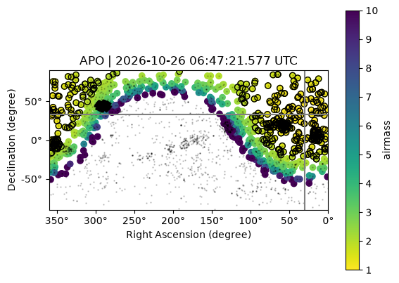
vi.PlanetGallery().build([unfiltered, filtered]);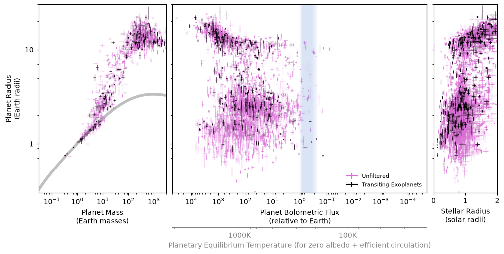
Make Target Sample
After looking at each of them one by one, let’s put all of those filtering criteria together.
targets = e[is_big * is_short * is_snr * is_up]
targets.label = "Observable?!"
targets
✨ Observable?! | 25 elements ✨vi.PlanetGallery().build([unfiltered, targets]);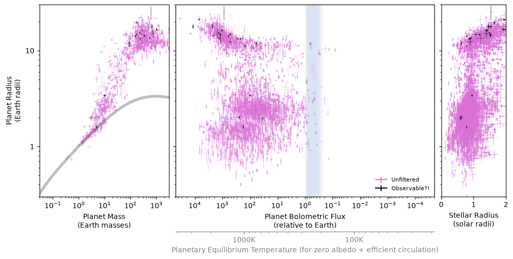
Let’s print out the names of the planets that made it through all our cuts.
print(targets.name())['GJ 9827 d' 'Gaia-2 b' 'HAT-P-1 b' 'HAT-P-19 b' 'HAT-P-47 b'
'HD 191939 b' 'HD 219134 b' 'K2-29 b' 'TOI-1408 b' 'TOI-1431 b'
'TOI-1518 b' 'TOI-2154 b' 'TOI-2578 b' 'TOI-3757 b' 'TOI-4145 A b'
'TOI-544 b' 'TOI-5806 b' 'TOI-6130 b' 'WASP-11 b' 'WASP-26 b' 'WASP-33 b'
'WASP-52 b' 'WASP-77 A b' 'WASP-93 b' 'XO-7 b']
Let’s also make a table that includes more useful information, like positions and transit ephemerides, which we could use as an input to plan an observing run.
table = targets.create_planning_table()
tableLet’s save that table out to a text file, and also make sure we can load it back in again.
observatory_string = observatory.name.replace(" ", "-")
date_string = local_midnight.iso.split()[0]
table.write(
    f"planets-to-observe-{observatory_string}-{date_string}.ecsv", overwrite=True
)
from astropy.io.ascii import read
read(f"planets-to-observe-{observatory_string}-{date_string}.ecsv")You can try filtering populations for your own devious and wonderful purposes, using whatever criteria you like!