🌊 Predicting Atmospheres

As a fun little application of exoatlas, we provide an example of how to estimate the probability a planet has an atmosphere according to the 3D cosmic shoreline model presented in Berta-Thompson, Wachiraphan, and Murray (2026, hereafter BTWM26). This page shows how to calculate atmosphere probabilities for planets and provides a few neat little visualizations.

from exoatlas import *

Calculate Atmosphere Probabilities for `exoatlas` Planets¶

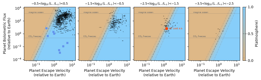
If you have an exoatlas population and simply want to calculate the probability its planets have atmospheres according to the shoreline model, then you can just call the probability_of_atmosphere() method attached to any exoatlas population. Behind the scenes, it will download posterior samples from Zenodo and use them to calculate atmosphere probabilities, marginalizing over the parameter uncertainties in the current version of the shoreline. Here’s the simplest version of what that looks like. Whenever we apply it, this shoreline accounts for the planet bolometric flux, planet escape velocity, and stellar luminosity in estimating the probability of atmospheric retention.

s = SolarSystem()
s.probability_of_atmosphere()

When we apply this shoreline model to the Solar System, everything but Mercury should have an atmosphere. When we apply it to exoplanets, it estimates different probabilities based on each system’s stellar and planetary environment.

e = TransitingExoplanets()

e['TRAPPIST-1'].probability_of_atmosphere()

e['LTT 1445Ab'].probability_of_atmosphere()

e['LHS 1140b'].probability_of_atmosphere()

Visualizing the BTWM26 Cosmic Shoreline¶

exoatlas has a few default built-in visualizing.ipynb to help show the shoreline across relevant parameter spaces. Because the shoreline is intrinsically 3D, these default visualizations show multiple slices of it, either in multiple panels or in an animation.

from exoatlas.visualizations import * 

# pick the name of the planet to highlight
planet_name = 'LTT1445Ab'

# create a subset population to highlight that one planet
highlight = e[planet_name]

# define a single panel of the visualization
m = ShorelineStandardMap()

# construct a grid of multiple slices
g = SliceGridGallery(m, N=4)

# add the planets to the panels
g.build([s, e, highlight])

# add embellishments to the plot, including probability 
g.refine()

# colorbar for probability
g.add_colorbar()

# save the figure
plt.savefig(f'shoreline-highlighting-{planet_name}.pdf')

from exoatlas.visualizations import * 

# pick the name of the planet to highlight
planet_name = 'LTT1445Ab'

# create a subset population to highlight that one planet
highlight = e[planet_name]

# define a single panel of the visualization
m = ShorelineStandardMap(order='vfL', )

# construct an animated grid of multiple slices
a = SliceAnimatedGallery(m, N=4, figsize=(4,4), dpi=300)

# make animation that steps through slices
a.animate([s, e, highlight], filename=f'animated-shoreline-highlighting-{planet_name}.gif')

# hide static figure
plt.close()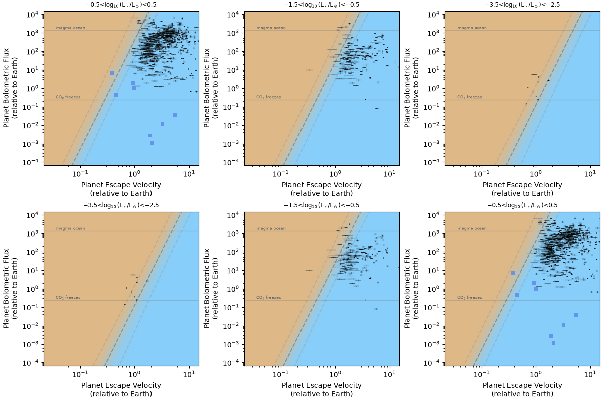

animated cosmic shoreline plot, with atmosphere probabilities appearing in sand and water colors

Direct Access to Shoreline Probabilities¶

If you want more nuanced control over what to do with the cosmic shoreline probabilities, you can create your own Shoreline object, which contains the posterior samples and can be used for various calculations. We’ll show how to do this, along with some of the background for the math used to calculate this probability.

from exoatlas.calculations.shoreline import Shoreline 

# automatically download default posterior
shore = Shoreline()

The probability model in BTWM26 defines a critical shoreline flux with

\log_{10} \left(\frac{f_{\sf shoreline}}{f_\oplus}\right) = \log_{10} \left(\frac{f_{\sf 0}}{f_\oplus}\right) + p \cdot \log_{10} \left(\frac{v_{\sf esc}}{v_{\sf esc, \oplus}}\right) + q \cdot \log_{10} \left(\frac{L_\star}{L_\odot}\right).

(1)

and a distance for a particular planet above that shoreline flux of

\Delta = \log_{10} \left(\frac{f_{\sf }}{f_\oplus}\right) - \log_{10}\left(\frac{f_{\sf shoreline}}{f_\oplus}\right) = \log_{10}\left(\frac{f}{f_{\sf shoreline}}\right)

(2)

and finally the probability of a planet having an atmosphere as

p_{\sf i} = P(A_{\sf i} = 1 | \mathbf{x}_{\sf i}, \boldsymbol{\theta} ) = \frac{1}{1+e^{\Delta_{\sf i}/w}}

(3)

where $f_0, p, q, w$ are the model parameters. We can retrieve point estimates of these parameters from the posterior.

point_parameters = shore.best_parameters()
point_parameters

{'log_f_0': 2.6166048266669573,
 'p': 5.903550424650916,
 'q': 1.1739214634550965,
 'ln_w': -1.396496413908506}

Let’s use those parameters to estimate the probability of planet receiving Earth-like flux with Earth-like escape velocity, but orbiting a much less luminous star with $L_\star = 10^{-2} L_\odot$ .

point_probability = shore.probability_of_atmosphere(log_f=0, log_v=0, log_L=-2, **point_parameters)
point_probability

np.float64(0.7476412243852795)

We can also use the samples of parameters to calculate the probability for many possible combinations of in the parameter posterior distribution. This would allow us to propagate the uncertainty in the parameters into the probability of a planet having an atmosphere.

sampled_parameters = shore.sampled_parameters()
sampled_parameters

samples_of_probability = shore.probability_of_atmosphere(log_f=0, log_v=0, log_L=-2, **sampled_parameters)
samples_of_probability

array([0.8956655 , 0.66789384, 0.83876477, 0.92185124, 0.59056938,
       0.77294455, 0.68460768, 0.68216085, 0.89351933, 0.59379868,
       0.84440551, 0.68283269, 0.8270999 , 0.55813355, 0.7805258 ,
       0.72355302, 0.88800367, 0.80098104, 0.7852569 , 0.55058969,
       0.63299954, 0.44115692, 0.69781734, 0.87487981, 0.75240876,
       0.53500072, 0.82150518, 0.88496797, 0.95727106, 0.63767673,
       0.36464743, 0.85983145, 0.48805844, 0.79250151, 0.82321434,
       0.90891369, 0.64325617, 0.7043401 , 0.91901637, 0.88308114,
       0.64225636, 0.78932838, 0.8776188 , 0.89533285, 0.85110821,
       0.67937925, 0.59726247, 0.75724515, 0.94276315, 0.88604936,
       0.40171358, 0.70265815, 0.68932824, 0.95807287, 0.66772353,
       0.64674912, 0.53279305, 0.64590355, 0.83915779, 0.93934855,
       0.72345792, 0.85025415, 0.45904688, 0.27921701, 0.74892662,
       0.66175621, 0.88645396, 0.62565873, 0.70324737, 0.87058458,
       0.76025817, 0.94312681, 0.58628657, 0.93904854, 0.85197129,
       0.80533394, 0.700235  , 0.96423037, 0.72491983, 0.73060644,
       0.78988913, 0.55998801, 0.7868839 , 0.83976391, 0.80629505,
       0.67957999, 0.70326125, 0.628526  , 0.64180152, 0.80349123,
       0.8256035 , 0.77266948, 0.52426649, 0.59118951, 0.6095214 ,
       0.63031488, 0.79578171, 0.36815797, 0.55878605, 0.60704679,
       0.90941439, 0.6996829 , 0.66553517, 0.74944444, 0.86773485,
       0.60274046, 0.91244177, 0.56275281, 0.88778244, 0.84866356,
       0.82865071, 0.7132766 , 0.73568001, 0.29616226, 0.6263698 ,
       0.9302668 , 0.64218885, 0.48752267, 0.87687758, 0.87742254,
       0.81136991, 0.97215878, 0.90208589, 0.53333418, 0.83270983,
       0.7173021 , 0.8734222 , 0.41793431, 0.89831568, 0.92595135,
       0.48432939, 0.78860661, 0.59141684, 0.52253659, 0.63509834,
       0.58325672, 0.77257477, 0.73788525, 0.49120162, 0.7286143 ,
       0.55472888, 0.52873822, 0.91292254, 0.87520928, 0.79943543,
       0.50953295, 0.7703639 , 0.89611537, 0.54722747, 0.79325866,
       0.47833171, 0.89736989, 0.91116007, 0.87279269, 0.74902353,
       0.55757113, 0.75919218, 0.45189472, 0.6323414 , 0.60213148,
       0.55394252, 0.67294451, 0.87727123, 0.78403735, 0.88078096,
       0.87288525, 0.73164487, 0.85353297, 0.91478222, 0.76817294,
       0.65552947, 0.65948239, 0.76025842, 0.83127015, 0.91689144,
       0.7152594 , 0.76172682, 0.67312016, 0.87173694, 0.81198958,
       0.20506863, 0.98149773, 0.49627758, 0.74931083, 0.60912082,
       0.79444437, 0.75040086, 0.56154275, 0.97147321, 0.59898962,
       0.84672632, 0.26653222, 0.90260212, 0.32536136, 0.74868823,
       0.83835131, 0.74505028, 0.62278867, 0.63976691, 0.59454755,
       0.68163468, 0.91867953, 0.77596574, 0.7882286 , 0.54746115,
       0.73654644, 0.71450402, 0.33364982, 0.87656732, 0.72938841,
       0.73527809, 0.63506984, 0.9419299 , 0.80872691, 0.83450209,
       0.79324784, 0.67989611, 0.93007074, 0.92582311, 0.83702012,
       0.74525658, 0.7197317 , 0.58492532, 0.44784898, 0.76346835,
       0.91460004, 0.8201526 , 0.8349902 , 0.4997777 , 0.80709111,
       0.95286366, 0.70156175, 0.9567002 , 0.60478174, 0.92935226,
       0.72650053, 0.77249767, 0.77962542, 0.42155009, 0.88089786,
       0.75851164, 0.8840345 , 0.68473881, 0.59852456, 0.75197041,
       0.30771603, 0.84725415, 0.79185389, 0.55825673, 0.77025497,
       0.60091829, 0.47321106, 0.36038478, 0.51280552, 0.54607138,
       0.57175296, 0.85806426, 0.86976716, 0.73061618, 0.99584291,
       0.7909615 , 0.35502683, 0.84695639, 0.54039976, 0.67011205,
       0.8926956 , 0.90120635, 0.61384935, 0.61912455, 0.88969272,
       0.90317858, 0.88281909, 0.33114398, 0.717674  , 0.69952619,
       0.31175001, 0.61186781, 0.90892337, 0.51043254, 0.75444475,
       0.60445824, 0.7502571 , 0.86003112, 0.68332713, 0.86005112,
       0.59150078, 0.68755098, 0.8505503 , 0.55229676, 0.87283005,
       0.73242934, 0.90032901, 0.77497038, 0.75156414, 0.72044502,
       0.24448569, 0.92011962, 0.79437088, 0.86716276, 0.77486847,
       0.58930972, 0.88177772, 0.6274732 , 0.90651913, 0.77657337,
       0.61570036, 0.92906876, 0.62482248, 0.87660067, 0.67952106,
       0.7216237 , 0.61365975, 0.80805354, 0.68155635, 0.80059837,
       0.75846955, 0.81271578, 0.72863066, 0.38965889, 0.22615199,
       0.41321938, 0.82015911, 0.79508717, 0.63840192, 0.41775484,
       0.88821346, 0.7079287 , 0.54162   , 0.8078957 , 0.50637534,
       0.86475023, 0.94055082, 0.67567721, 0.59962617, 0.81388989,
       0.62526676, 0.83913092, 0.89295018, 0.64093679, 0.83870175,
       0.84645949, 0.70832367, 0.78804957, 0.47550659, 0.82862733,
       0.81859213, 0.54999981, 0.83160422, 0.80347889, 0.97157176,
       0.83748578, 0.81183505, 0.77592513, 0.82760128, 0.81332491,
       0.76230831, 0.9160827 , 0.65447522, 0.66581698, 0.41185862,
       0.97297831, 0.64238254, 0.57394033, 0.3652367 , 0.58615538,
       0.44706483, 0.77847295, 0.67562928, 0.62571858, 0.83355313,
       0.48864967, 0.58033044, 0.3998398 , 0.78328573, 0.67025583,
       0.9539464 , 0.81746744, 0.62796786, 0.74196218, 0.74384217,
       0.5222424 , 0.92125751, 0.70644049, 0.57885212, 0.89663856,
       0.66483879, 0.638856  , 0.74965886, 0.70277353, 0.88402174,
       0.90085568, 0.73812971, 0.92018165, 0.76588583, 0.89566465,
       0.82973281, 0.81483436, 0.73924689, 0.88649095, 0.98290857,
       0.33563599, 0.7728711 , 0.74379511, 0.8480315 , 0.65077932,
       0.72661506, 0.80396746, 0.78144923, 0.93521594, 0.52634989,
       0.79271975, 0.49051273, 0.97714574, 0.84309972, 0.94584307,
       0.72943281, 0.39703099, 0.62220603, 0.7591166 , 0.85754765,
       0.96161875, 0.81532032, 0.87631814, 0.95837762, 0.76277234,
       0.56136311, 0.76890179, 0.52118531, 0.68385013, 0.74685615,
       0.8585243 , 0.82227703, 0.68978328, 0.58559502, 0.79777311,
       0.73865123, 0.60921897, 0.5613904 , 0.61385145, 0.92695536,
       0.41913685, 0.88838225, 0.51551261, 0.70706574, 0.78877026,
       0.91535835, 0.42322371, 0.573873  , 0.65589085, 0.98238973,
       0.75116251, 0.62205567, 0.91035136, 0.59833133, 0.21111776,
       0.9673113 , 0.66844298, 0.42208937, 0.64549203, 0.8483595 ,
       0.86749513, 0.72237868, 0.51478958, 0.74277161, 0.81679638,
       0.80258293, 0.7795646 , 0.62273805, 0.73387885, 0.78770128,
       0.71713393, 0.64013551, 0.3583115 , 0.79873879, 0.69136136,
       0.75932772, 0.79668575, 0.92046508, 0.4889975 , 0.43137134,
       0.79682539, 0.86868167, 0.60996103, 0.39640938, 0.86261616,
       0.95309541, 0.54235984, 0.77602203, 0.96683388, 0.9021267 ,
       0.88282505, 0.65214571, 0.72395652, 0.41839483, 0.84697199,
       0.82261386, 0.8160655 , 0.50986321, 0.58456638, 0.85419703,
       0.69023771, 0.67212516, 0.38031471, 0.83992093, 0.85612374,
       0.66609931, 0.90270123, 0.57248447, 0.84380113, 0.58124957,
       0.9075155 , 0.60998154, 0.78260096, 0.85945918, 0.68067576,
       0.81713026, 0.86558089, 0.83898701, 0.53940761, 0.66598613,
       0.92022765, 0.91130541, 0.73670584, 0.35886332, 0.50247683,
       0.85326105, 0.77258497, 0.97291977, 0.83494925, 0.88374484,
       0.56639314, 0.83956769, 0.48670787, 0.31715503, 0.96845082,
       0.63187191, 0.816273  , 0.91710508, 0.81546637, 0.39323221,
       0.89723138, 0.67609837, 0.44720137, 0.68636229, 0.47298916,
       0.75105738, 0.57336704, 0.78775935, 0.65010794, 0.91966735,
       0.56944914, 0.88600942, 0.79531988, 0.91650965, 0.85709943,
       0.31946948, 0.76716775, 0.79421277, 0.67102378, 0.71467515,
       0.80551216, 0.67287963, 0.52507201, 0.84351789, 0.83137171,
       0.58706233, 0.7051407 , 0.75338324, 0.50076104, 0.92813972,
       0.96639971, 0.76447036, 0.08918453, 0.94664696, 0.63379633,
       0.66506919, 0.86990666, 0.53033877, 0.68350469, 0.81236482,
       0.51256286, 0.72348056, 0.95448109, 0.66897162, 0.73937445,
       0.52982756, 0.9493493 , 0.84487945, 0.44056025, 0.83604899,
       0.70499202, 0.87686622, 0.79193475, 0.77972528, 0.39231058,
       0.94641272, 0.77172877, 0.50896661, 0.93567904, 0.40968052,
       0.34514174, 0.68683019, 0.89921448, 0.5916851 , 0.92283194,
       0.92830539, 0.95055444, 0.71752187, 0.62993754, 0.94878479,
       0.80206432, 0.69375732, 0.65828084, 0.50853772, 0.8175467 ,
       0.45349919, 0.91684712, 0.86415002, 0.73084725, 0.80534874,
       0.78781616, 0.92014275, 0.73134399, 0.85137203, 0.74242637,
       0.95130923, 0.7693876 , 0.65434716, 0.77612636, 0.51803282,
       0.87576187, 0.76200115, 0.83591908, 0.57261345, 0.58180787,
       0.40487024, 0.47079486, 0.52558434, 0.523309  , 0.82683342,
       0.88589987, 0.74443658, 0.75807728, 0.51997576, 0.60522349,
       0.67758747, 0.7442041 , 0.83990477, 0.60620616, 0.57823684,
       0.6855779 , 0.67731044, 0.9154426 , 0.62098958, 0.95813994,
       0.68477618, 0.84036229, 0.76219396, 0.72292596, 0.92487656,
       0.78260152, 0.59520724, 0.94130235, 0.31568789, 0.4976473 ,
       0.59036844, 0.79555316, 0.66241473, 0.55391688, 0.86878556,
       0.94725289, 0.70419156, 0.60026962, 0.65059624, 0.68086135,
       0.53394255, 0.90541484, 0.84918841, 0.95958238, 0.80849591,
       0.84656266, 0.48695914, 0.38469293, 0.93213843, 0.95081471,
       0.77568535, 0.58560883, 0.39529302, 0.51802434, 0.71690111,
       0.78970852, 0.88754487, 0.89866602, 0.69203564, 0.52681231,
       0.66731234, 0.95221086, 0.90377578, 0.85492531, 0.88150967,
       0.94196181, 0.53269775, 0.47161497, 0.75472993, 0.74284298,
       0.85303707, 0.92469612, 0.87925044, 0.38109328, 0.87741477,
       0.73142933, 0.76776796, 0.61041694, 0.71611461, 0.49684054,
       0.72393248, 0.85279631, 0.28697275, 0.70929101, 0.40438799,
       0.33928717, 0.84903018, 0.91624013, 0.53514582, 0.60384759,
       0.71435682, 0.94552192, 0.48409605, 0.68804231, 0.9704286 ,
       0.81952061, 0.29919472, 0.44022716, 0.76985009, 0.45560318,
       0.71532176, 0.83342027, 0.61278747, 0.8282922 , 0.43414109,
       0.72448245, 0.76681514, 0.74407709, 0.76612629, 0.66725503,
       0.67231419, 0.62985211, 0.63281179, 0.93510442, 0.92274579,
       0.93469918, 0.69973274, 0.89893338, 0.96639743, 0.74754023,
       0.80245894, 0.59869166, 0.67778636, 0.67439452, 0.93178372,
       0.76443187, 0.88011155, 0.7880614 , 0.86575942, 0.57908906,
       0.87047392, 0.94860712, 0.85872233, 0.72949844, 0.91865645,
       0.7277195 , 0.57874805, 0.69317321, 0.74229615, 0.95338619,
       0.86229753, 0.81173351, 0.8020857 , 0.7774758 , 0.56529066,
       0.77495768, 0.80378304, 0.78116836, 0.61640072, 0.43759415,
       0.67270496, 0.64085731, 0.63936986, 0.97821878, 0.61768661,
       0.41176912, 0.88556483, 0.73687999, 0.465451  , 0.63725691,
       0.81442716, 0.44246184, 0.70321884, 0.83525406, 0.91844151,
       0.79383013, 0.85876816, 0.78091289, 0.8621368 , 0.81805939,
       0.73310157, 0.7871904 , 0.79487484, 0.62924861, 0.51931653,
       0.80730125, 0.83960787, 0.89857613, 0.54471758, 0.78709971,
       0.44200382, 0.66867559, 0.75580648, 0.88473001, 0.80791635,
       0.73376818, 0.53269285, 0.90073299, 0.71606437, 0.62686398,
       0.93202734, 0.83138783, 0.56747392, 0.93884214, 0.44414092,
       0.60734826, 0.46352835, 0.7397748 , 0.82642753, 0.67161263,
       0.76825023, 0.61915569, 0.79801147, 0.52443079, 0.52698379,
       0.8811928 , 0.70756606, 0.94264586, 0.70285913, 0.39618469,
       0.87440491, 0.55076823, 0.77240635, 0.58522686, 0.73670429,
       0.29561999, 0.74525941, 0.78257978, 0.61351226, 0.55937921,
       0.72819663, 0.89674006, 0.75941142, 0.93395891, 0.72968585,
       0.66413341, 0.65709716, 0.77571756, 0.90681833, 0.79176705,
       0.84363714, 0.36021257, 0.81090909, 0.71139341, 0.69047303,
       0.77792817, 0.61770459, 0.83450961, 0.82027351, 0.74240158,
       0.73692937, 0.7097167 , 0.57912573, 0.64477068, 0.85244435,
       0.83829647, 0.63452038, 0.54487196, 0.92614421, 0.7041437 ,
       0.99201358, 0.34212732, 0.81347865, 0.92048406, 0.59303251,
       0.73471045, 0.80049257, 0.91185526, 0.88587464, 0.70791194,
       0.61795032, 0.53173276, 0.80386785, 0.74714873, 0.81403532,
       0.56546148, 0.77539901, 0.98271435, 0.26752342, 0.60977895,
       0.43660435, 0.80963408, 0.93524375, 0.73737095, 0.72299286,
       0.74150896, 0.73949151, 0.86954413, 0.73354989, 0.52633182,
       0.15943096, 0.90387203, 0.94584299, 0.64977971, 0.60543163,
       0.4781065 , 0.81064863, 0.89929015, 0.4460138 , 0.72377844,
       0.89217509, 0.41734285, 0.67165921, 0.8091181 , 0.89318023,
       0.78552951, 0.56340403, 0.6383198 , 0.81901964, 0.43506625,
       0.50967827, 0.65122367, 0.29651024, 0.96825788, 0.59740188,
       0.75810209, 0.82171703, 0.89319252, 0.84359595, 0.76602602,
       0.86819275, 0.63302541, 0.5935795 , 0.70917834, 0.62980761,
       0.69364978, 0.45483768, 0.75533397, 0.86727394, 0.76235217,
       0.66426508, 0.8085311 , 0.48312878, 0.76513969, 0.62785426,
       0.62489045, 0.47296718, 0.83127067, 0.9316948 , 0.41722674,
       0.69758051, 0.83088362, 0.62693513, 0.74863477, 0.9436785 ,
       0.53904085, 0.84757208, 0.67578825, 0.68500858, 0.76321792,
       0.92499089, 0.9336931 , 0.64431317, 0.71234471, 0.8995383 ,
       0.40459206, 0.708116  , 0.59002378, 0.91363176, 0.80045646,
       0.7607937 , 0.5260331 , 0.76774483, 0.42825216, 0.58963444,
       0.77113166, 0.86702717, 0.90078134, 0.73351054, 0.66107994,
       0.6824813 , 0.84411013, 0.67444771, 0.66681156, 0.8616581 ])

plt.hist(samples_of_probability, alpha=0.3, label='with parameter uncertainty')
plt.axvline(point_probability, label='without parameter uncertainty')
plt.legend(frameon=False)
plt.xlabel('Probability of Atmosphere')
plt.yticks([])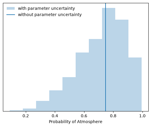

([], [])

The .calculate_probability_of_atmosphere_from_posterior_samples function provides a simple wrapper to calculate summary statistics for the atmosphere probability, accounting for the shoreline parameter uncertainties. It provides three numbers: the median probability of an atmosphere, the lower $1\sigma$ confidence interval, and the upper $1\sigma$ confidence interval. By default, these are returned as three numbers; with the latex=True keyword flag, they can be returned as a tidy LaTeX-friendly string.

shore.calculate_probability_of_atmosphere_from_posterior_samples(log_f=0, log_v=0, log_L=-2)

(np.float64(0.7197926118635868),
 np.float64(0.17146451174796884),
 np.float64(0.16739234741182962))

shore.calculate_probability_of_atmosphere_from_posterior_samples(log_f=0, log_v=0, log_L=-2, latex=True)

['{latexify_confidence_interval(m*100, l*100, u*100)}\\%']

Standard exoatlas populations can also provide access to distributions of calculated atmosphere probabilities. Simply provide the distribution=True keyword to a population’s .probability_of_atmosphere() method, as shown below. For Mars, the distribution of probabilities incorporates the uncertainties in the shoreline parameters. For the exoplanet, it includes both the uncertainties in the shoreline parameters and the uncertainties propagated from the substantial uncertainties on the intrinsic planet parameters.

plt.figure(figsize=(8,3))

histkw = dict(bins = np.linspace(0, 1), alpha=0.5)
p = e['LTT1445Ab'].probability_of_atmosphere(distribution=True)
plt.hist(p.distribution[0], label='LTT1445Ab', **histkw)

p = s['Mars'].probability_of_atmosphere(distribution=True)
plt.hist(p.distribution[0], label='Mars', **histkw)

plt.legend(frameon=False)
plt.xlabel('Probability of Atmosphere');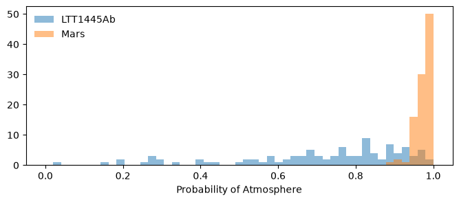

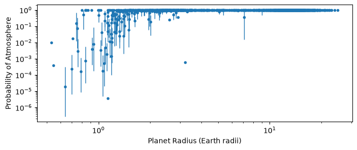
These distributions are used when calculating uncertainties on the derived atmosphere probability. Read more about uncertainties for subtles about how these uncertainties get propagated.

# calculate atmosphere probabilities *and* asymmetric uncertainties
x = e.radius()
y = e.probability_of_atmosphere()
lower, upper = e.get_uncertainty_lowerupper('probability_of_atmosphere')

plt.figure(figsize=(8,3))
plt.scatter(x, y, marker='.')
plt.errorbar(x, y, [lower, upper], elinewidth=1, linewidth=0)
plt.xscale('log'); plt.yscale('log');
plt.xlabel('Planet Radius (Earth radii)') 
plt.ylabel('Probability of Atmosphere');

🌊 Predicting Atmospheres

Calculate Atmosphere Probabilities for exoatlas Planets¶

Visualizing the BTWM26 Cosmic Shoreline¶

Direct Access to Shoreline Probabilities¶

Further Reading¶

Calculate Atmosphere Probabilities for `exoatlas` Planets¶